Negative Binomial Distribution

Contents

1 Introduction
2 Differences between Binomial Random Variable and Negative Binomial Random Variable
3 Detailed Example – 1
4 Probability Distribution
- - 4.0.1 X = Number of failures that precede the rth success.
5 Detailed Example – 2
6 Expected Value and Variance
7 Geometric Distribution
- - 7.0.1 Formula
    - 7.0.1.1 References

Introduction

Negative Binomial Distribution (also known as Pascal Distribution) should satisfy the following conditions;

The experiment should consist of a sequence of independent trials.
Each trial should have only 2 outcomes. That is Success (S) or Failure (F).
Success Probability θ should be constant from trial to trial.
The experiment should be continued until the occurrence of r total successes. Here r is a specified positive integer.

In the Binomial Distribution, we were interested in the number of Successes in n number of trials. But in the Negative Binomial Distribution, we are interested in the number of Failures in n number of trials. This is why the prefix “Negative” is there.

Differences between Binomial Random Variable and Negative Binomial Random Variable

Negative Binomial Random Variable	Negative Binomial Random Variable
Fixed No. of trials.	Trials are not fixed, random.
No. of successes is not fixed.	No. of failures are fixed.

Detailed Example – 1

Consider an experiment where we roll a die until the face 6 turns upwards two times.

Here;

Our trials are independent. That means turning 6 face upwards on one trial does not affect whether or 6 face turns upwards on the next trials.
Each trial only has 2 outcomes.
Success probability is constant. 1/6 for every trial.
The experiment is continued until the 6 face turns upwards 2 times.

Probability Distribution

X = Number of failures that precede the r^th success.

(1) $\begin{equation*} \boxed{f_X{(x)}=\binom{x+r-1}{x}\theta^{r}(1-\theta)^x} \end{equation*}$

Terminology;

x – value of the Random Variable X
r – r^th success. (no. of failures = (r-1))
θ – Success probability

Detailed Example – 2

A researcher is interested in examining the relationship between students’ mental health and their exam marks. For this, he wishes to conduct interviews with 5 students.

θ = Probability of a randomly selected student agrees to sit for the interview

θ = 0.2

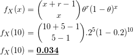
What is the probability that 15 students should be asked before 5 students are found to agree to sit for the interview?

(2) $\begin{align*} f_X{(x)}&=\binom{x+r-1}{x}\theta^{r}(1-\theta)^x \\ f_X{(10)}&=\binom{10+5-1}{5-1}\0.2^{5}(1-0.2)^{10}\\ f_X{(10)}&= \underline{\textbf{0.034}} \end{align*}$

Expected Value and Variance

Expected number of trials until first success is;

(3) $\begin{align*} \theta=\dfrac{1}{trials}\Longrightarrow{trials=\dfrac{1}{\theta}} \end{align*}$

Therefore, expected number of failures until first success is;

(4) $\begin{align*} \dfrac{1}{\theta}-1 = \dfrac{1-\theta}{\theta} \end{align*}$

Hence, we expect $\dfrac{r(1-\theta)}{\theta}$ failures before the r^th success.

Therefore,

(5) $\begin{align*} E(X)&=\dfrac{r(1-\theta)}{\theta} \\ V(X)&=\dfrac{r(1-\theta)}{\theta^2} \end{align*}$

Geometric Distribution

This is a special case of Negative Binomial Distribution where r=1

That means, we are interested in finding number of trials that is required for a single success.

Example :
Tossing a coin until it lands on heads.

Formula

(6) $\begin{align*} X~geometric(\theta) \\ f_X{(x)}&=(1-\theta)^x\theta \end{align*}$

References

Probability and Statistics for Engineering and the Sciences 8th Edition by Jay. L. Devore
https://stattrek.com/ – This site features very high quality statistics content!