Introduction
Hello, guys welcome all of you to my series of lessons on Regression Analysis. In this post, we will discuss about Simple Linear Regression. So, without further ado, let’s jump into the content!
Simple Linear Regression is the method how we analyze the relationship between two quantitative variables. The result of Simple Linear Regression is a linear regression equation that can be used to make predictions.
What are the Variables in Simple Linear Regression?
One variable, which is often denoted by ‘x’ is called the “Predictor Variable”. This is also referred to as “Independent” or “Explanatory” variable in some texts.
Other variable, which is denoted by ‘y’ is called the “Response Variable”. The response variable is also known as the “outcome” or “the dependent variable”
Example for SLR
We can build up an equation that gives the value of annual sales (Y) when the money spent on advertising (X) is recorded.
Why “Simple”
Simple Linear Regression (also referred to as SLR) is called “Simple” because we only study one predictor variable here. Whereas, in Multiple Linear Regression, we study about two or more predictor variables.
Why Linear?
The word ‘Linear’ is used here to express that this relationship can be denoted by a straight line. In other words, the said relationship can be expressed in the form of ;
y = mx + c
Further, the word ‘Linear’ tells you that the regression parameters are entered in a linear fashion to the above equation. (i.e, no x2, x3 etc.)
Types of Relationships
In the following lessons, we study only about Statistical Relationships. We are not learning about Deterministic Relationships.
Deterministic Relationships
Deterministic Relationship is a relationship where an equation exactly describes the relationship between 2 variables.
Example;
Relationship between ‘kilograms’ and ‘pounds’
1 Pound = 0.45 kilograms
Statistical Relationships
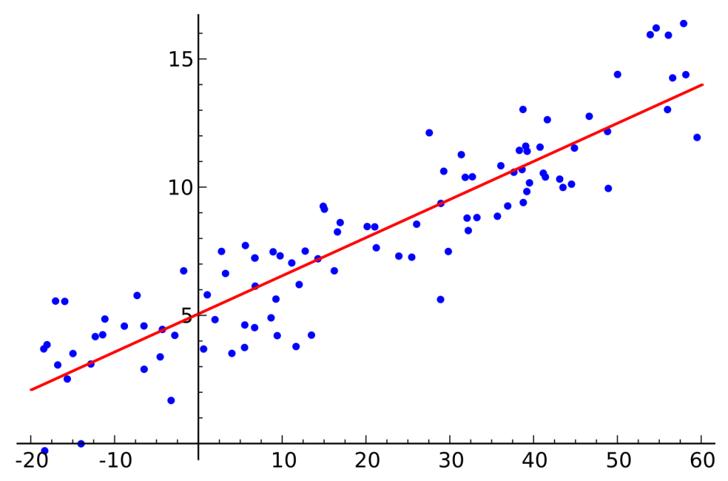
Here, the relationship between the variables is not accurate.

In the above Scatter Plot, we can see that there is a relationship between the two variables. But it is not perfect. Yes, the plot exhibits some trend, but there is also ‘scatter’. Therefore, it is a Statistical Relationship.
You can discover more about these two relationships by following this link.
Simple Linear Regression Model
Let us talk about the example we discussed under the statistical relationships. You already saw the scatterplot relating to the data above.
Since you now know what is a Statistical Relationship, you know that the exact value of sales cannot be predicted for a given amount of advertising expenditure. This is the nature of a ‘statistical relationship’.
Even if we include several other variables into the Regression Equation, we cannot predict the sales revenue 100% accurately.
Why cannot we predict exactly?
This is because there are always some variations in sales as a result of random reasons.
Population Regression Line
To do accurate predictions, we must know the Population Regression Line. To draw a Population Regression Line, we must collect data from everyone in the population. But this is practically impossible. Therefore, we take a sample from the data to estimate the population regression line.
Simple Linear Regression Model
Take the Average Statistics Marks for students with a GPA of 1. Similarly, take the Average Statistics marks for students with GPA 2,3, and 4. We can plot a graph by using these data. That graph can be summarized as follows;

 represents the mean of Y variable for a given value of X. This is called the “conditional mean”.
The line that connects the conditional means is known as the true population regression line.
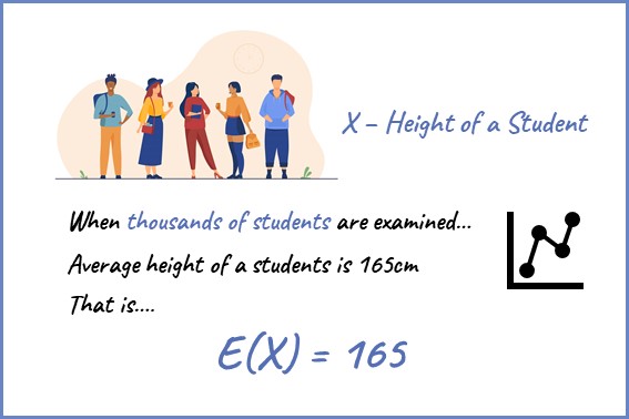
The term E(Y|X = x) means the Expected Value of Y given the value of Random Variable X, equals the value of x. You can find more about the Expected Value of a Random Variable by clicking on the link here.
Also, it is clear that every student’s Statistics marks will not equal the mean . There will be some errors.

The blue color dots are the actual marks of students. The gap between the regression line and data points is the error
This means Student’s response y is a function of the linear trend  plus some error
Therefore, the relationship between a response variable Y and predictor variable X can be represented as;

The above equation is called the Sample Regression Equation.
Sample Regression Equation
As explained earlier, we always deal with samples because of the practical difficulties in handling a population. Therefore in Regression Analysis also we estimate the Population Regression Line using a Sample Regression Equation.
We have to estimate the population parameters ( ) using our sample regression equation. To do that, we use a method called “Ordinary Least Squares (OLS)”. In some texts, this is referred to as “Method of Least Squares”.
Next Article
Estimation of Best Fitting Line
Related Pages