Estimation of Best Fitting Line

Sample Linear Regression Model

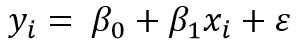
x_i is the predictor value for experimental unit i

y_i is the response value for the experimental unit i

An “experimental unit” is the object on which the observation is made.

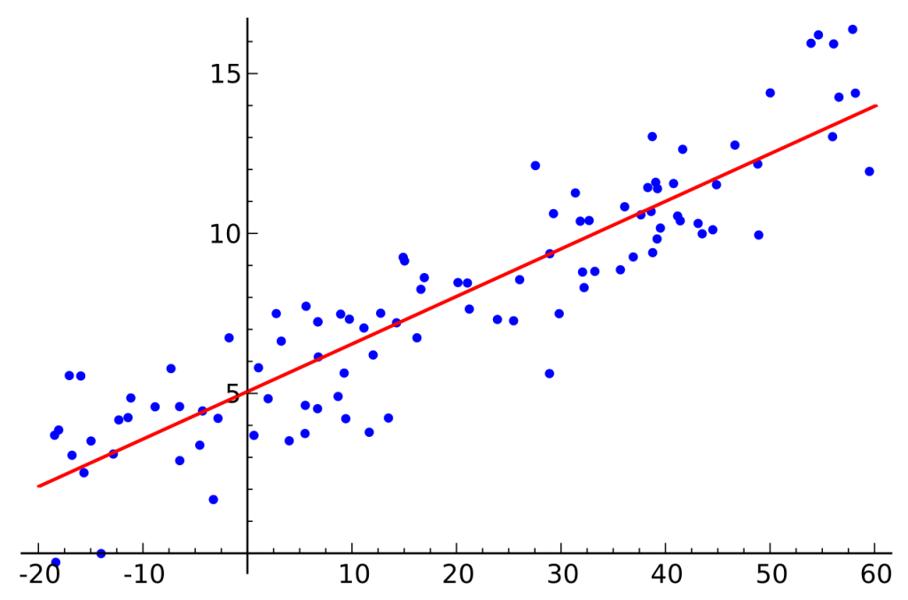
Best Fitting Line

We can find the best fitting line using the Method of Least Squares. This method was invented by the German mathematician Carl Friedrich Gauss.

We can estimate Beta 0 and Beta 1 using this method

What is Ordinary Least Squares Method?

In the Ordinary Least squares method we estimate the model parameters such that the variance is kept at a minimum. In other words, It minimizes the sum of the squares of the differences between the observed response variable (dependent variable) and those predicted by our regression equation.

Estimation of β₀ and β₁

We know that our error terms is the difference between the observed value and the predicted value. Therefore, we have to subject the error term in the Sample Linear Regression.

Then we have to take the sum of squares of all error terms in our sample and differentiate it with respect to β₀ and β₁

The least squares estimators of β₀ and β₁ say and , must satisfy

and

Simplifying the above two equations yields

The above two equations are called the least-squares normal equations.

When we solve the above two equations we get answers for and

And

where

We can write the equation for the slope in a simpler way like this;

AND

Therefore, we can write conveniently as;