In our previous post, we described to you how to handle the variables when there are categorical predictors in the regression equation. If you missed that, please read it from here. In this post, we will do the Multiple Linear Regression Analysis on our dataset. Also if you don’t have the dataset, please download it from here.
First let’s see some scatter plots to get an idea about the relationship between variables.
Given below is the scatterplot of charges vs age with the categorical variables “smoker” and “gender” as group variables

Here you can see there is a slight positive relationship between age and insurance charges. In fact, if you run a correlation analysis for the above data, you will get a correlation coefficient of 0.297. We can see smoking males and females have high insurance charges. Also, almost all the non-smoking males and females have insurance charges around 10,000$. Only one observation is above that limit.
Now let’s generate the scatterplot of charges vs BMI with the categorical variables “smoker” and “sex”
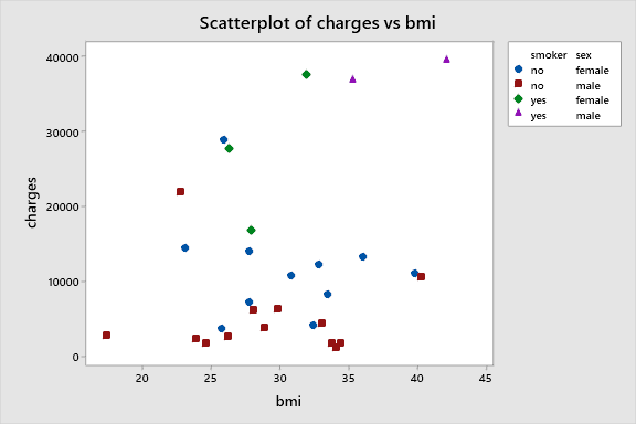
Here there is no relationship between BMI and charges. The data points are scattered everywhere. Correlation analysis outputs the correlation coefficient as 0.2.
The scatterplot below represents the relationship between age vs BMI.
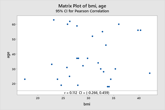
We can clearly see that there is no relationship between the two variables. All the data points are scattered everywhere. The correlation coefficient of 0.112 testifies our claim
Okay, now let’s jump into the Regression Analysis.
We first conduct Simple Linear Regression Analysis with each Independent variable with the Dependent Variable. Then we move on to the full regression model.
Since it takes so much space to display all our regression results, I have summarized the results in the following table
| Model | F | P-Value | S | R-sq (adj) | R-sq (Pred) |
| Age | 2.61 | 0.118 | 11271.2 | 5.44% | 0% |
| bmi | 1.43 | 0.243 | 11503.5 | 1.50% | 0% |
| bmi,age | 1.86 | 0.176 | 11251.2 | 5.77% | 0% |
| bmi,sex | 1.58 | 0.225 | 11356.8 | 4.00% | 0% |
| age,sex | 1.33 | 0.282 | 11456.9 | 2.30% | 0% |
| age,smoke | 39.88 | 0 | 5963.69 | 73.53% | 64.03% |
| bmi,smoke | 20.93 | 0 | 7445.25 | 58.74% | 50.98% |
| bmi,smoke,age | 25.6 | 0 | 6078.94 | 72.49% | 59.27% |
| bmi,age,sex | 1.28 | 0.303 | 11421 | 2.91% | 0% |
| full model | 19.71 | 0 | 6048.29 | 72.71% | 57.10% |
From the above table, you can see that Single Variable models are out of the question. Age, Smoke model is significant with the lowest regression error. It has the highest R-sq (adj) and R-sq (pred) values too. Those values are even better than the full regression model. Therefore we can conclude that the regression equation with age and smoke variables is the best model that fits the data.