Importing and Getting to Know Data
Hello dear friends! Today we are going to see how to handle/impute missing values in a simple dataset using R Statistical Programming Language.
For this, we are going to use the “airquality” dataset that comes with R.
First, let’s import our dataset
> data("airquality")For convenience, we create a copy of the data frame and name it as “aq”
> aq<-data.frame(airquality)Now, we are going to check the data types of each column. This is not necessary for the data cleaning process, but I thought it would be better to give you some extra knowledge as well. We use “sapply” function to view the data types of each column.
> sapply(aq, class) Ozone Solar.R Wind Temp Month Day
"integer" "integer" "numeric" "integer" "integer" "integer" All the variables in our data set are quantitative variables. Variables “Month” and “Day” should be categorical variables.
aq$Day <- factor(aq$Day, levels=c(1:31), ordered=TRUE)
aq$Month <- factor(aq$Month, levels=5:9, labels=month.abb[5:9], ordered=TRUE)
You can view the dimension of your data frame from the following command.
> dim(aq)This returns a vector of the dimensions of your data frame. That is how many rows and columns are there in the data frame $(rows, columns)$
[1] 153 6Identifying Missing Values
Let’s have a sneak peek on our dataset
> head(aq) Ozone Solar.R Wind Temp Month Day
1 41 190 7.4 67 May 1
2 36 118 8.0 72 May 2
3 12 149 12.6 74 May 3
4 18 313 11.5 62 May 4
5 NA NA 14.3 56 May 5
6 28 NA 14.9 66 May 6You can clearly see that there are missing values in our data set. $(“NA” values represent missing values here. It is an acronym for “Not Available”)$
We’ll create a summary of our data frame as well
> summary(aq) Ozone Solar.R Wind Temp Month Day
Min. : 1.00 Min. : 7.0 Min. : 1.700 Min. :56.00 May:31 1 : 5
1st Qu.: 18.00 1st Qu.:115.8 1st Qu.: 7.400 1st Qu.:72.00 Jun:30 2 : 5
Median : 31.50 Median :205.0 Median : 9.700 Median :79.00 Jul:31 3 : 5
Mean : 42.13 Mean :185.9 Mean : 9.958 Mean :77.88 Aug:31 4 : 5
3rd Qu.: 63.25 3rd Qu.:258.8 3rd Qu.:11.500 3rd Qu.:85.00 Sep:30 5 : 5
Max. :168.00 Max. :334.0 Max. :20.700 Max. :97.00 6 : 5
NA's :37 NA's :7 (Other):123 The above summary confirms that there are missing values in our dataset. Precisely, 37 missing values in the column “Ozone” and 7 missing values in the column “Solar.R”. Therefore, we have to find a way to deal with these missing values.
We need to have an exact idea about the missing values in our data set. To create meaningful analysis and insights, we need to clean our data well.
More Insight to Missing Values
According to the summary output we produced above, there are missing value in only 2 columns. Other columns are free from missing values.
Generally, we leave out any variable with over 5% missing values. To get the percentage of missing values in each column, we create a custom function;
percentmissing<-function(aq){
  (colSums(is.na(aq))/nrow(aq))*100
}
percentmissing(aq)
When we run the above function in the R console, we get the following output;
> percentmissing(aq)
    Ozone   Solar.R      Wind      Temp     Month       Day
24.183007  4.575163  0.000000  0.000000  0.000000  0.000000
According to the above output, there are nearly 25% missing values in “Ozone” column and 4.5% missing values in “Solar.R” column.
Obviously we have a problem with the “Ozone” column since there are nearly 25% missing values.
Missing Value Pattern
Let’s have a better understanding about the pattern of missing values. For this, we can use “mice” package. MICE stands for Multivariate Imputation by Chained Equations.
> library(mice)
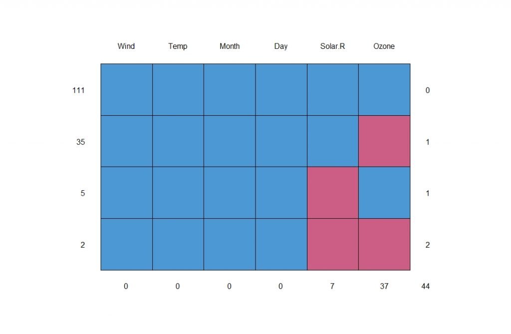
> md.pattern(aq)When we run the above code, we get the following output;
    Wind Temp Month Day Solar.R Ozone
111    1    1     1   1       1     1  0
35     1    1     1   1       1     0  1
5      1    1     1   1       0     1  1
2      1    1     1   1       0     0  2
       0    0     0   0       7    37 44
We can interpret the above table in the following manner;
There are 111 rows which are complete (free from missing values). 35 Rows are missing the value for “Ozone” column, 5 Rows are missing the value for “Solar.R” column and 2 Rows are missing the value for “Ozone” and “Solar.R” columns. Altogether we have 44 data points which are incomplete.
You can get a better understanding about the pattern from the plot below;
We know that there are 153 rows in our data set. From the above chart, there are 111 complete observations. That means nearly 72% of our data is complete. We can visualize that insight as follows;
Visualization of Missing Values
We use the VIM package (VIM stands for – Visualization and Imputation for Missing Values)
> library(VIM)
> aggr(aq, combined = FALSE, numbers = TRUE)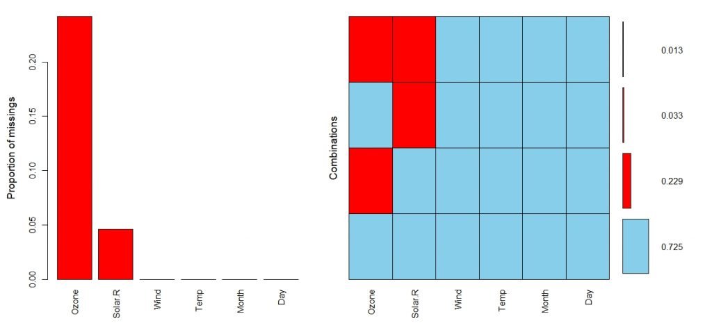
In the above plot, blue color areas are the areas where the observations are complete. The vertical axis represent the proportion of data. Therefore, nearly 72.5% of data is complete.
Imputation of Missing Values
Early I told you that if a variable is missing over 5% of data, we leave it out. But here if we do that, we will be losing over 24% of our data. That is not acceptable. Therefore we have to look for another imputation method. We can use column mean to replace missing data but it is not accurate. But for the “Solar.R” column we can use mean imputation as well since there are only 7 missing values. But why use biased methods when we have more accurate methods?
We can impute these missing values using “mice” function. It imputes each missing variable with a separate model. It will choose the best imputation method considering the type of each variable (factor, integer etc).
> impute<-mice(aq,m=3,seed=500)
> print(impute)
The above function outputs a “mids” object. It means Multiply Imputed Data Set. In the function arguments, we have given m=5 which means the number of multiple imputations is 3. The default value of m is 5. We have set the seed to 500, but that is optional.
 iter imp variable
  1   1  Ozone  Solar.R
  1   2  Ozone  Solar.R
  1   3  Ozone  Solar.R
  2   1  Ozone  Solar.R
  2   2  Ozone  Solar.R
  2   3  Ozone  Solar.R
  3   1  Ozone  Solar.R
  3   2  Ozone  Solar.R
  3   3  Ozone  Solar.R
  4   1  Ozone  Solar.R
  4   2  Ozone  Solar.R
  4   3  Ozone  Solar.R
  5   1  Ozone  Solar.R
  5   2  Ozone  Solar.R
  5   3  Ozone  Solar.R
Class: mids
Number of multiple imputations:  3
Imputation methods:
  Ozone Solar.R    Wind    Temp   Month     Day
  "pmm"   "pmm"      ""      ""      ""      ""
PredictorMatrix:
        Ozone Solar.R Wind Temp Month Day
Ozone       0       1    1    1     1   1
Solar.R     1       0    1    1     1   1
Wind        1       1    0    1     1   1
Temp        1       1    1    0     1   1
Month       1       1    1    1     0   1
Day         1       1    1    1     1   0
So the above is our output. We can see that there are 5 iterations of 3 different imputations. The imputation method of each variable is also stated. Here “pmm” (predictive mean matching) is used for both the variables “Ozone” and “Solar.R”.
PMM basically chooses the most correlated variable for the variable with missing value and predicts the missing values using regression techniques. Note that this is a very brief explanation and the real algorithm is more complex. You can learn more about predictive mean matching algorithm from here.
Let’s have a look at some imputed values.
impute$imp$Ozone
1  2   3
5   13  1  18
10  28 46  16
25  46 65  49
26  18 13   8
27  18  9  18
Here I have displayed only the first 5 imputed values only because it takes larger space to display all 37 imputed values.
Explanation of Imputed Values
For the 5th data point (row), we have 3 imputed values for “Ozone” 13, 1 and 18. If we had used mean to impute this missing data point, we would have had 37 which is the mean of the “Ozone” column. You can see that it is nowhere near any of the 3 imputed values.
In this data set, there is no correlation between the variables. If there were, this would be very clear. Nevertheless, it is clear that our imputation technique is way better than the mean imputation.
Completing the Data
We can use any of the 3 imputations to complete the data.
Let’s use the 2nd imputation;
> complete(impute,1)Now we get a completed data set with more accurately imputed missing values.
So, that’s mostly it about missing value imputation. Please note that imputation of missing value is a very crucial part of the data cleaning process and you have to do it in the most accurate way possible. Otherwise, it can badly affect our predictions or whatever the outputs we produce from our data.
Hope you guys got a grab on how to handle missing values using R and don’t forget to subscribe to our blog and share this among your friends and colleagues!