We did a basic Multiple Linear Regression Analysis in our previous post. If you missed that, please click the link and refer it. Here we go one step forewards by adding categorical variables into the regression equation. Let’s see how to do that!
What is a Categorical Variable?
A Categorical Variable has two or more categories. They are also called as Qualitative Variables. Examples for Categorical Variables are “gender”, “marital status” etc.
What is a Dummy Variable?
When we have one or more Categorical Variables in our regression equation, we express them as “Dummy Variables”. For a variable with n categories, there are always (n-1) dummy variables. Dummy Variables are also called as “Indicator Variables”
Example of a Dummy Variable:-
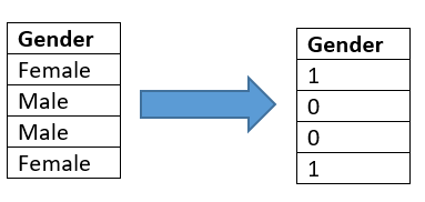
Say we have the categorical variable “Gender” in our regression equation. We can represent this as 0 for Male and 1 for Female.

Let’s jump into our problem
The dataset that we are going to use here is called “insurance”. You can download the dataset from here. We are interested in predicting insurance charges. Most probable factors which determine the insurance charges for a certain individual are listed.
We have 6 Independent Variables here.
| Variable | Type |
|---|---|
| Age | Quantitave |
| Sex | Categorical (2) |
| BMI | Quantitative |
| Children | Quantitative |
| Smoker | Categorical (2) |
| Region | Categorical (4) |
In the above table, I have listed all the Predictor Variables and their type. Also, no. of categories mentioned within parenthesis in front of each categorical variable.

Let’s code each categorical variable into indicator (dummy) variables
Sex
Male -> 0 Female -> 1
Smoker
Yes ->1 No ->0
| Region | Code |
| North East | 0 |
| North West | 1 |
| South East | 2 |
| South West | 3 |
Region
We have four categories here (n = 4). Therefore we need (4-1) = 3 Indicator Variables here.
As a rule of thumb, we code variables according to the alphabetical order.
| age | sex | bmi | children | smoker | region |
| 19 | 1 | 27.9 | 0 | 1 | 3 |
| 18 | 0 | 33.77 | 1 | 0 | 2 |
| 28 | 0 | 33 | 3 | 0 | 2 |
| 33 | 0 | 22.705 | 0 | 0 | 1 |
| 32 | 0 | 28.88 | 0 | 0 | 1 |
| 31 | 1 | 25.74 | 0 | 0 | 2 |
| 46 | 1 | 33.44 | 1 | 0 | 2 |
| 37 | 1 | 27.74 | 3 | 0 | 1 |
| 37 | 0 | 29.83 | 2 | 0 | 0 |
| 60 | 1 | 25.84 | 0 | 0 | 1 |
Number of Possible Regression Equations
For a moment, assume that there is only one Categorical Predictor variable named ‘Gender’ and One Quantitative Predictor named ‘Age’.
Our regression equation look like follows;

Since gender can only take values 1 and 0, whenever gender = 0, regression equation consist of only beta 0 and beta 1.
Therefore it is clear that, whenever categorical variables are present, the number of regression equations equals the product of the number of categories. In our example above we have 3 categorical variables consisting of all together (4*2*2) 16 equations.
Now we have done the preliminary stage of our Multiple Linear Regression Analysis. That is we have finished coding our variables. Now we have to do the Regression Analysis. We that using Minitab Software.
Note that we have truncated this data set and dropped some columns to make our regression analysis simple.
Please refer the next post for analysis
