Introduction
Usually when conducting experiments, all treatment combinations are assigned to all the blocks. Thus, they are called “complete” designs. But in the real world, this might not be the case always. Due to resource constraints and physical size of blocks, the experimenter is forced to use randomized block designs where every treatment is not present in every block. These designs are known as Randomized Incomplete Block Designs.
In these designs, a sample of treatments selected and randomly assigned to a block.
Balanced Incomplete Block Designs $(BIBD)$
At instances where all treatment comparisons are of equal importance, a balanced design is a must. In such cases, experiment should be designed in such a way that any pair of treatment combinations should occur the same number of times as any other pair.
Hence, a Balanced Incomplete Block Design can be defined as an incomplete block design where any two treatments appear an equal number of times.
Statistical Analysis of Balanced Incomplete Block Designs
Suppose that there are t number of treatments and k, $(k<t)$ is the block size.
Each block has to be appeared r times in the design.
Number of blocks can be calculated as follows;
Total number of experimental units $(n)$ = bk = tr
Number of blocks $(b)$ = tr/k
In practice, t and k are fixed and r is changed accordingly.
Number of times each pair of treatments appear in the same block $(λ)$ can be defined as;
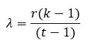
This is also known as “order of comparison”.
If t = b, design is said to be symmetric.
For a feasible design, λ should be an integer.
Worked Example
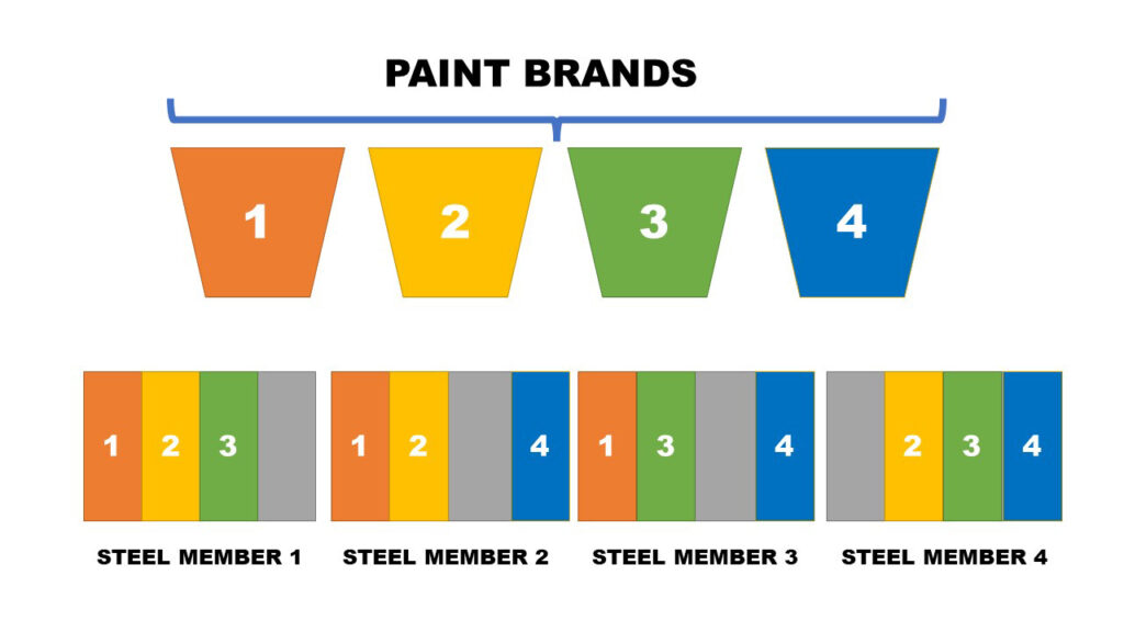
A civil engineer thinks that the thickness of corrosion generating on a steel member at a coastal area depends on the brand of marine paint applied on its surface. To test this, he designs an experiment where he uses 4 brands of marine paints.
There can be slight variations in the chemical composition of steel members according to the manufacturer. Because of this, engineer decides to use samples from 4 major steel manufacturers who sends steel to Canada as blocks.
4 Steel “wide flange” members which were of length 6m were used as blocks in the experiment. Initially it was planned to apply the 4 brands of paint on each 6m long steel member by dividing a single steel member into 4 sections.
But unfortunately, the surface area of a block $(i.e., steel member)$ is not large enough to apply all the 4 brands of paints. The surface area of a single block was only sufficient to apply 3 brands of paints. Hence, the engineer decided to conduct a Balanced Incomplete Block Design.
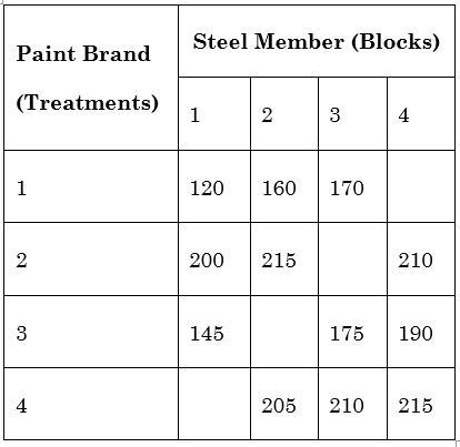
The Balanced Incomplete Design for this experiment along with the observations recorded is shown in the following table.
Corrosion thickness is measured in microns $(1 micron = 0.001 mm)$
In this case, t = 4, r = 3, k = 3
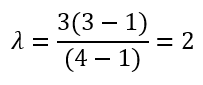
Hence λ is an integer, a balanced design exists.
Interpretation of Results
ANOVA
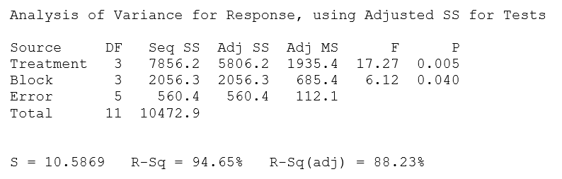
From the ANOVA Table, it can be concluded that the treatments are significant at 5% level of significance. That is, the brand of Marine Paint has an effect on the amount of corrosion on a Steel Surface. Also, R-Squared value is over 94.65%. That means over 94% of the variability in the data is explained by this model.
Graphs
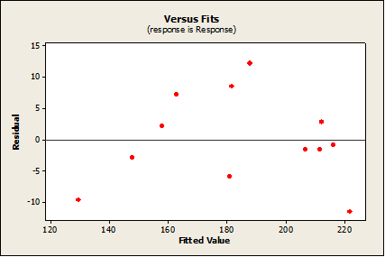
In this analysis, several assumptions have been made;
- Residuals are Independent
- Residuals are Normally Distributed with 0 mean and constant variance
From the Residuals vs Fitted values plot, it is clearly seen that residuals vary around 0 on a horizontal band and there is no clear pattern visible. Hence it can be inferred that mean of the residuals is 0 and the variance is constant.
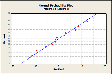
From the Normal Probability plot, the data points are positioned in very close proximity to the normal probability line, hence the normality assumption is satisfied.
Grouping Information
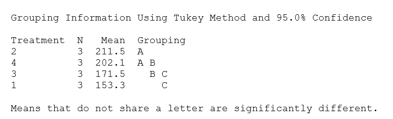
Mean of treatment 2 is higher than the rest of the treatments. There is no significant difference between treatments 2 & 4, 4 & 3, 3 & 1.
Tukey 95% Confidence Intervals
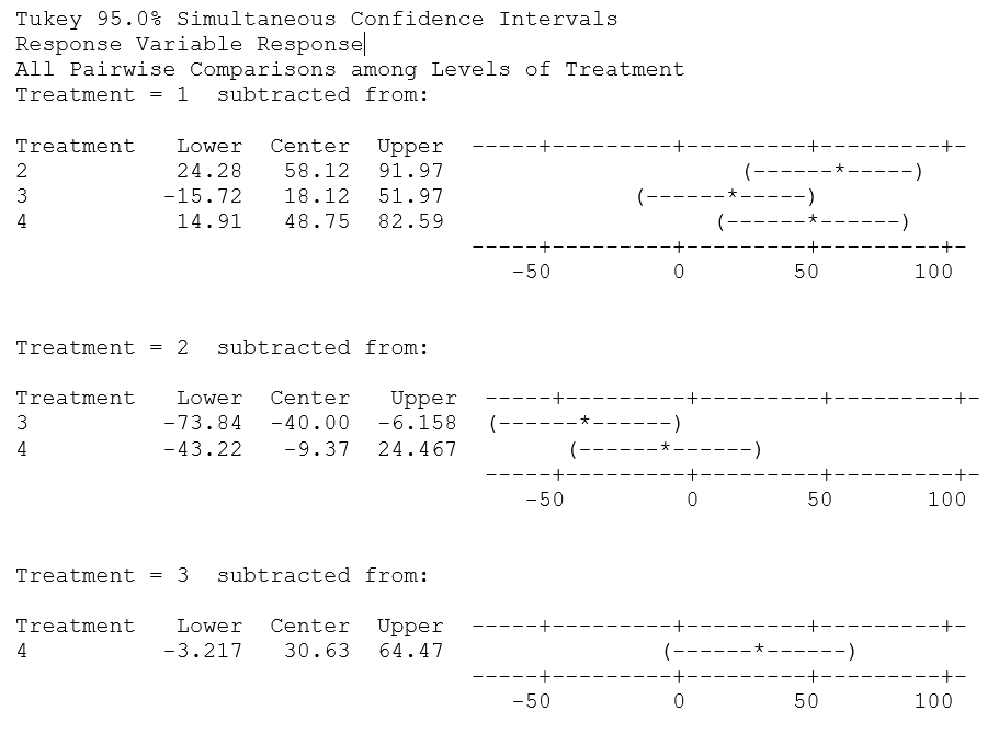
Confidence interval for the difference between means of treatment 2 and 1 does not contain 0. That implies those are statistically significant. Hence, it can be concluded that the mean difference would be at least 24.28 microns and at most it can be 91.97 microns.
Similarly, confidence interval for the difference between means of treatment 4 and 1 does not contain 0. That implies those are statistically significant. Hence, it can be concluded that the mean difference would be at least 14.91 microns and at most it can be 82.59 microns.
Same logic applies for the treatment difference of treatment 3 & 2. Here, the mean difference would be at most 73.84 microns and at least 6.158 microns.
Rest of the confidence intervals for the treatment mean differences $(1 & 3, 4 & 2, 4 & 3)$ contain 0 $(they vary from positive to negative)$. Hence, they are not statistically significant. Therefore, in this experiment they are not of any use.
Tukey Simultaneous Tests
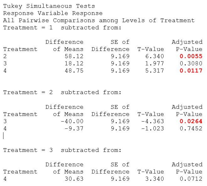
Results obtained from the Tukey comparison tests also confirms the above interpretations. There are 3 p-values which are statistically significant (marked in red in the output)
References
Design and Analysis of Experiments by Douglas C. Montgomery (8th Edition)